Stochastic optimisation
A lot of problems arising in machine learning are actually optimisation problems of the form
min_x [F(x) = \sum_{i=1}^N f_i(x)] where f_i(x) is a smooth function corresponding to the loss on the i-th training sample.
There are two common ways of solving this optimisation problem. First of all, one could use a general method for minimising a general smooth function. A standard method for this task is a quasi-Newton method such as BFGS (or L-BFGS). One of the main reasons why these methods are popular is that approximating the Hessian of the function allows the method to converge very fast. Another advantage is that there is no need to manually adjust any hyperparameters.
However, these methods need to compute the value and gradient of the full function F(x) at each step. To compute these two quantities one essentially needs to sum the values and gradients of all the functions f_i(x) which is a very expensive operation since the number of functions N is usually very large.
The second way is to use a stochastic optimisation method such as stochastic gradient descent (SGD). While a general quasi-Newton method treats the function F(x) as a black-box function, SGD exploits the fact that F(x) is actually a sum of other similar functions f_i(x). As a result, the method only needs to compute the gradient of some f_i(x) at each iteration. It makes the iteration of SGD much cheaper than that of a quasi-Newton method: while the latter makes one step, SGD makes N steps.
Each of these two approaches has its advantages and disadvantages. On the one hand, if just a few passes over the entire training set (say, 5) are feasible, then quasi-Newton makes only a few steps and approximates the Hessian poorly. In this case, SGD is most certainly the preferred method. On the other hand, if several dozen more passes can be made, then quasi-Newton methods typically improve their approximation of the Hessian and outperform SGD.
However, a serious drawback of SGD is its high sensitivity to hyperparameters (e.g., learning rate). Depending on the choice of hyperparameters the rate of convergence of SGD may change significantly. Even though there are situations when certain procedures can be used to automatically adjust these hyperparameters, these situations are rather uncommon. So, in practice the user often has to choose the hyperparameters manually.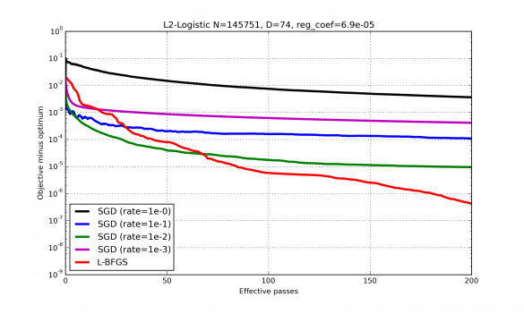 Example of typical convergence of SGD and quasi-Newton. At the beginning SGD decreases the objective much faster and so it is the method of choice when only several passes over the entire training set are feasible. If many more passes are possible, then quasi-Newton outperforms SGD. Also one can see high sensitivity of SGD to the learning rate.
In this project we are developing an optimisation method which combines the two approaches mentioned above. It is being designed to approximate the function curvature by maintaining a quadratic model of the objective function and at the same time to have low cost of each iteration. As well as that, the method should not make the user set any hyperparameters.
![]()
Have you spotted a typo?
Highlight it, click Ctrl+Enter and send us a message. Thank you for your help!
To be used only for spelling or punctuation mistakes.